The queue at the gate: why waiting time doesn't grow the way you think

Every terminal, depot and weighbridge in the corridor has a gate, and every gate has a queue. The mathematics of that queue has been understood since Erlang worked out telephone congestion in 1917 — and it behaves in a way that surprises almost everyone the first time they see it. Waiting time does not grow in proportion to traffic. It creeps, then it explodes. This analysis builds the model, validates it two independent ways, and shows what it means for anyone who runs — or waits at — a gate.

Two random processes, one predictable disaster

A gate is a service system: trucks arrive, each takes time to process, and anyone who arrives while the lanes are busy waits. Two features make it tractable. Arrivals from many independent operators behave like a Poisson process — random, uncoordinated, clumpy. And processing times vary around a mean. A gate with c lanes then behaves as the classic M/M/c queue, whose average wait has a closed-form answer known since Erlang.

The term that matters is the denominator: (c·μ − λ) — the gate's spare capacity. As demand approaches capacity it goes to zero and the wait explodes — not gradually, hyperbolically. This is why a gate that felt fine on Tuesday can fall apart on Thursday with only slightly more traffic.

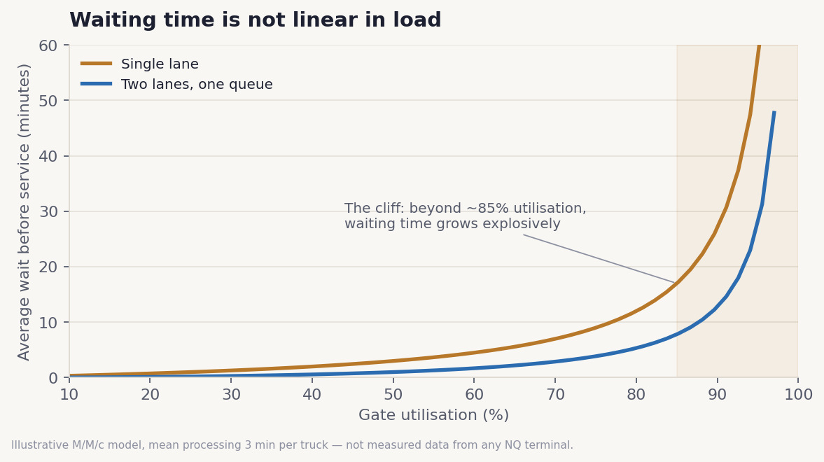
Fig. 1 — Average wait against utilisation for a single lane and a two-lane shared queue (mean processing 3 min/truck). At 60% utilisation the single lane averages under 3 minutes of waiting; at 85% it averages 17; at 95% it averages 57. The last 10 points of utilisation cost more than the first 80 combined.

"Busy all day" is fragility, not efficiency: at 95% utilisation there is no slack for the clumping random arrivals guarantee. And averages deceive — congestion must be analysed at the peak hour, not the daily mean.

Two independent methods, one answer

A model that has not been checked is a guess with equations. The Erlang-C results were therefore cross-examined with a discrete-event simulation: 200,000 synthetic arrivals per scenario, served by whichever lane frees first — no queueing formulas anywhere in the code. If the two methods disagree, one of them is wrong.

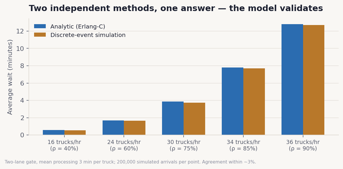
Fig. 2 — Analytic result against simulation across five load levels on a two-lane gate. The two methods agree within about 3% everywhere, including deep in the congested region. The model is validated.

Cutting waits without pouring concrete

The instinctive response to congestion is capital: add a lane. The theory says two cheaper levers come first. Pooling: two lanes fed by one shared queue outperform two separate single-lane queues at identical demand, because a shared queue never leaves one lane idle while trucks wait at the other. Variability reduction: waiting is driven by randomness as much as load — Kingman's approximation ties the wait to arrival variability. A slot system doesn't change how many trucks come; it changes how randomly they come, and the queue responds as if capacity had been added.

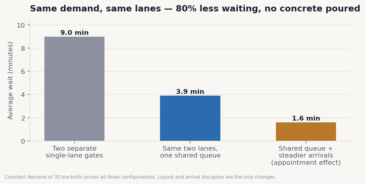
Fig. 3 — Same demand (30 trucks/hr), same two physical lanes. Merging the queues cuts the average wait 57%; smoothing arrivals on top of that brings the total reduction to roughly 80%. Neither step requires construction.

Pool first, smooth second, build last. Concrete is the most expensive and slowest lever — and the model shows most of the available improvement is organisational.

Five moves, in order

Model: M/M/c queue solved with the Erlang-C formula; cross-validated with an independent discrete-event simulation (200,000 arrivals per scenario; agreement within ~3%). Arrival smoothing modelled by reducing the coefficient of variation of inter-arrival times from 1.0 to 0.25. Assumptions and limits: stationary demand within the modelled hour, exponential service times, no balking or lane-switching, homogeneous trucks. Real gates have peaks, breakdowns and mixed traffic — so treat the figures as directional and the shape of the behaviour as exact. The model deliberately uses illustrative parameters rather than unverified operational data from any local terminal, in line with the Review's editorial rule: if a number cannot be traced to a primary source, it is not presented as fact.

Theory sources: A.K. Erlang, "Solution of some problems in the theory of probabilities" (1917) — the Erlang-C formula. J.D.C. Little, "A proof for the queuing formula L = λW" (1961). J.F.C. Kingman, "The single server queue in heavy traffic" (1961) — the variability approximation. All results reproduced independently for this analysis.